![[Deep Learning] Attention 메커니즘](https://img1.daumcdn.net/thumb/R750x0/?scode=mtistory2&fname=https%3A%2F%2Fblog.kakaocdn.net%2Fdna%2FEKRQh%2FbtqEBdNhIZX%2FAAAAAAAAAAAAAAAAAAAAAA9k1xVHiCFkgZOLEpx2Ag8LAvgYY1GqMj2S09wnOw9K%2Fimg.png%3Fcredential%3DyqXZFxpELC7KVnFOS48ylbz2pIh7yKj8%26expires%3D1769871599%26allow_ip%3D%26allow_referer%3D%26signature%3DrZqOGIIlcfJtNdVPXn%252FAJcfOEWA%253D)
[Deep Learning] Attention 메커니즘
Attention Mechanism 이란?
기존의 RNN, 즉 recurrent model에서는 문장의 순차적 특성을 유지한다. 하지만, 두 정보 사이의 거리가 멀 때 해당 정보를 이용하지 못하는 문제가 발생한다. 이 문제는 Long-term dependency problem라고 한다. 다시말해 recurrent model은 학습 시 t번째 hidden state를 얻기 위해 t-1번째 hidden state가 필요하다(=과거 정보를 이용한다.) 즉, 순서대로 계산되어야 하기 때문에 병렬 처리가 불가능하고 속도라 느리다(Parallelization).
이를 해결하기 위한 방법인 Attention이란, 모델이 중요한 부분에 집중(attention)하게 만드는 기법이다. Attention에서는 decoder에서 출력 단어를 예측하는 매 시점마다 encoder에서의 전체 입력 문장을 다시 참고한다. 이때, 동일한 비율로 참고하는 것이 아닌, 해당 시점에서 예측해야 할 단어와 연관 있는 입력 단어 부분에 좀 더 집중해서(attention)해서 보게된다.
Neural Machine Translation (Seq2seq Model 사용)
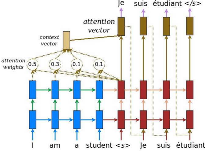
Attention mechanism은 대표적으로 Nerual Machine Translation에 사용된다. 그 예시는 아래 이미지와 같다. 아래 이미지를 보면 Je라는 출력을 예측하기 위해 encoder에서의 전체 입력 문장을 context vector를 통해 참고한다. 즉, 차례대로 살펴보면, 우선 파란색 박스 부분은 encoder, 빨간색 박스 부분은 decoder이고 갈색은 classify layer를 나타낸다. 파란색 박스에 들어오는 입력 "I", "am", "a", "student"는 각각이 계산되서 attention weights를 만든다. 이를 종합한게 context vector인데 출력을 예측하기 위해 매번 이 context vector와 빨간색 박스에서 나오는 각각의 hidden state를 concat(연결해서 합침)해서 attention vector를 구한다. 이 attention vector를 이용해 각각 "Je", "suis", "etudiant", "</s>"를 예측하게 된다.
간단하게 얘기하면 Translation(번역)을 할때, "Je suis etudiant"에서 "etudiant" 예측시, 연관성이 높은 "student"라는 단에서 좀더 주목하게 만들게 되는 방식이다.
Attention Function
Attention을 함수로 표현하면 아래와 같다.
Attention(Q, K, V) = Attention Value

위의 식에서 Q, K, V는 각각 query, key, value를 나타내는데 여기서 key와 value는 흔히 말하는 dictionary 방식에서의 key value 값을 의미한다.
이 함수는 Q, K, V가 입력값으로 주어졌을 때,
- 먼저 query(Q)에 대해 모든 key(K)와의 유사도를 각각 구한다.
- 이 유사도를 key와 mapping되어 있는 각각의 value(V)에 반영한다.
- 그 후, 유사도가 반영된 value를 모두 더해서 return하면 이 return 된 값이 attention value가 된다.
Code
위 과정을 식으로 나타내보자.
(h = key, s = query)
초록색 박스는 query가 모든 key와의 유사도를 구하는 식이다.
노란색 박스는 그 유사도를 얼마나 반영할지의 값을 구하는 식이다.
주황색 박스는 구한 반영 비율만큼 value를 반영해서 attention에 적용하는 과정이다.

Attention mechanism을 코드로 나타내면 다음과 같다.
# Trainable parameters
w_omega = tf.Variable(tf.random_normal([hidden_size, attention_size], stddev=0.1))
b_omega = tf.Variable(tf.random_normal([attention_size], stddev=0.1))
u_omega = tf.Variable(tf.random_normal([attentionsize], stddev=0.1))

with tf.name_scope('v'):
	# Applying fully connected layer with non-linear activation to each of the B*T timestamps
    # the shape of 'v' is (B, T, D)*(D, A)=(B, T, A), where A=attention_size
    v = tf.tanh(tf.tensordot(inputs, w_omega, axes=1) + b_omega)

    # For each of the timestamps, its vecotr of size A from 'v' is reduced with 'u' vector
    vu = tf.tensordot(v, u_omega, axes=1, name='vu') # (B, T) shape
    alphas = tf.nn.softmax(vu, name='alphas') # (B, T) shape

    # Output of (Bi-)RNN is reduced with attention vector: the result has (B, D) shape
    output = tf.reduce_sum(inputs * tf.expand_dims(alphas, -1), 1)
Neural Machine Translation (seq2seq) Code
그렇다면 Seq2seq + attention 모델에서의 Q, K, V를 살펴보자. 이 모델에서 Q, K, V는 다음과 같다.
- Q : Decoder의 t-1 셀에서의 은닉 상태
- K : 모든 Encoder 셀의 은닉 상태들
- V : 모든 Encoder 셀의 은닉 상태들
아래 코드는 seq2seq 모델에 attention을 적용하기 전의 코드이다.
import tensorflow as tf
import numpy as np

# S : 디코딩 입력의 시작을 나타냄
# E : 디코딩 출력의 끝을 나타냄
# P : 현재 배치 데이터의 time step 크기가 작은 경우 빈 시퀀스를 채우는 것을 나타냄
#	ex) to -> ['t', 'o', 'P', 'P']

char_arr = [c for c in 'SEPabcdefghijklmnopqrstuvwxyz단어나무놀이소녀키스사랑']
num_dic = {n: i for i, n in enumerate(char_arr)}
dic_len = len(num_dic)

# training data for translation
seq_data = [['word', '단어'], ['wood', '나무'], ['game', '놀이'], ['girl', '소녀'], ['kiss', '키스'], ['love', '사랑']]

def make_batch(seq_data):
    input_batch = []
    output_batch = []
    target_batch = []

    for seq in seq_data:
    	# 인코더 셀의 입력값, 입력단어의 글자들을 한글자씩 떼어 배열로 만든다.
        input = [num_dic[n] for n in seq[0]]
        # 디코더 셀의 입력값, 시작을 나타내는 S 심볼을 맨 앞에 붙여준다.
        output = [num_dic[n] for n in ('S' + seq[1])]
        # 학습을 위해 비교할 디코더 셀의 출력값. 끝나는 것을 알려주기 위해 마지막에 E를 붙인다.
        target = [num_dic[n] for n in (seq[1] + 'E')]

        input_batch.append(np.eye(dic_len)[input])
        output_batch.append(np.eye(dic_len)[output])
        # 출력값만 one-hot 인코딩이 아님 (sparse_softmax_cross_entropy_with_logits 사용)
        target_batch.append(target)

    return input_batch, output_batch, target_batch

# 옵션 설정
learning_rate = 0.01
n_hidden = 128
total_epoch = 100
#입력과 출력의 형태가 one-hot 인코딩으로 같으므로 크기도 같다.
n_class = n_input = dic_len

## 신경망 모델구성
# seq2seq 모델은 인코더의 입력과 디코더의 입력의 형식이 같다.
# [batch size, time, steps, input size]
enc_input = tf.placeholder(tf.float32, [None, None, n_input])
dec_input = tf.placeholder(tf.float32, [None, None, n_input])
# [batch size, time steps]
targets = tf.placeholder(tf.int64, [None, None])

# 인코더 셀을 구성한다.
with tf.variable_scope('encode'):
    enc_cell = tf.nn.rnn_cell.BasicRNNCell(n_hidden)
    enc_cell = tf.nn.rnn_cell.DropoutWrapper(enc_cell, output_keep_prob=0.5)
    outputs, enc_states = tf.nn.dynamic_rnn(enc_cell, enc_input, dtype=tf.float32)

# 디코더 셀을 구성한다.
with tf.variable_scope('decode'):
    dec_cell = tf.nn.rnn_cell.BasicRNNCell(n_hidden)
    dec_cell = tf.nn.rnn_cell.DropoutWrapper(dec_cell, output_keep_prob=0.5)

    # seq2seq 모델은 인코더 셀의 최종 상태값을 디코더 셀의 초기 상태값으로 넣어주는 것이 핵심
    outputs, dec_states = tf.nn.dynamic_rnn(dec_cell, dec_input, initial_state=enc_states, dtype=tf.float32)

model = tf.layers.dense(outputs, n_class, activation=None)
cost = tf.reduce_mean(tf.nn.sparse_softmax_cross_entropy_with_logits(logits=model, labels=targets))
optimizer = tf.train.AdamOptimizer(learning_rate).minimize(cost)

## 신경망 모델 학습
sess = tf.Session()
sess.run(tf.global_variables_initializer())

input_batch, output_batch, target_batch = make_batch(seq_data)

for epoch in range(total_epoch):
    _, loss = sess.run([optimizer, cost], feed_dict={enc_input: input_batch, dec_input: output_batch, targets: target_batch})

    print('Epoch:', '%04d' % (epoch + 1), 'cost =', '{:.6f}'.format(loss))

print('최적화 완료')

## 번역 테스트
# 단어를 입력받아 번역 단어를 예측하고 디코딩하는 함수
def translate(word):
	# 이 모델은 입력값과 출력값 데이터로 [영어단어, 한글단어]를 사용하지만, 예측시에는 한글단어를 알지 못하므로
	# 디코더의 입출력값을 의미 없는 값인 P 값으로 채운다. ['word', 'PPPP']
    seq_data = [word, 'P' * len(word)]
    input_batch, output_batch, target_batch = make_batch([seq_data])

    # 결과가 [batch size, time step, input]으로 나오기 때문에
    # 2번째 차원인 input차원을 argmax로 취해 가장 확률이 높은 글자를 예측 값으로 만든다.
    prediction = tf.argmax(model, 2)

    result = sess.run(prediction, feed_dict={enc_input: input_batch, dec_input: output_batch, targets: target_batch})

    # 결과 값인 숫자의 인덱스에 해당하는 글자를 가져와 글자 배열을 ㅁ나든다.
    decoded = [char_arr[i] for i in result[0]]

    # 출력의 끝을 의미하는 'E' 이후의 글자들을 제거하고 문자열로 만든다.
    end = decoded.index('E')
    translated = ''.join(decoded[:end])

    return translated

print('\n=== 번역 테스트 ===')

print('word ->', translate('word'))
print('wodr ->', translate('wodr'))
print('love ->', translate('love'))
print('loev ->', translate('loev'))
print('abcd ->', translate('abcd'))
사용한 모델은 이후 추가 예정
'CS > Deep Learning' 카테고리의 다른 글
| [Deep Learning] Recurrent Neural Network(RNN) (0) | 2020.05.20 |
|---|---|
| [Deep Learning] 합성곱 신경망 (Convolution Neural Network, CNN) (0) | 2020.05.12 |
| [Deep Learning] 가중치 초기화 & Check Point (0) | 2020.05.11 |
| [Deep Learning] Auto-Encoder (1) | 2020.04.24 |
| [Deep Learning] Optimizer (1) | 2020.04.19 |